译 - Scalable Bloom Filters

《Scalable Bloom Filters》 这篇论文讲述了一种布隆过滤器的变体实现方式，通过将预设的误判率分配给多个子布隆过滤器来约束整体的一个误判率情况，并且可以通过新增子布隆过滤器来实现对存储元素数量的调节，以满足初始容量无法准确估计的情况，论文中详细介绍了在不同的误判率变化率以及布隆过滤器容量变化率的情况下，存储空间等的使用情况。目前了解到的，RedisBloom 和 TairBloom 都参考了这篇论文实现了各自的布隆过滤器。

摘要

Bloom Filters provide space-efficient storage of sets at the cost of a probability of false positives on membership queries. The size of the filter must be defined a priori based on the number of elements to store and the desired false positive probability, being impossible to store extra elements without increasing the false positive probability. This leads typically to a conservative assumption regarding maximum set size, possibly by orders of magnitude, and a consequent space waste. This paper proposes Scalable Bloom Filters, a variant of Bloom Filters that can adapt dynamically to the number of elements stored, while assuring a maximum false positive probability.

布隆过滤器已查询成员资格时的误判概率为代价，提供了对数据集的高效空间存储能力。过滤器的大小需要依据要存储的元素数量和所需的误报概率来提前确定，如果不允许增加误报率，就不能存储额外的元素。这通常会导致我们对数据集合的大小做一个保守的估计（可能是数数量级的差异），这就会导致空间的浪费。本文提出了可扩展的布隆过滤器，它是布隆过滤器的一个变体，在保证最大误判率的情况下能够动态适应可存储元素的数量。

Keywords: Data Structures, Bloom Filters, Distributed Systems, Randomized Algorithms

关键词：数据结构、布隆过滤器、分布式系统、随机算法

1、介绍

Bloom filters [1] provide space-efficient storage of sets at the cost of a probability of false positive on membership queries. Insertion and membership testing in Bloom filters implies an amount of randomization, since elements are transformed using one-way hash functions. Testing for the presence of elements that have actually been inserted in the filter will always give a positive result; there are no false negatives. On the contrary, there is always some probability of false positives: elements that have not been inserted into the filter can erroneously pass the membership test.

布隆过滤器[1]通过以成员查询的误判率为代价，提供了高效的空间来存储数据集。由于元素是使用单向哈希函数转换，因此布隆过滤器中的插入和成员测试（查询）意味着一定程度的随机化。查询一个元素是否已经插入总是能得到明确的答案，不会存在假阴性（误判）。对应的，总是有一些误判的情况：没有被插入过滤器的元素被错误地通过成员资格测试（被误判已经插入）。

An important property of Bloom filters is the linear relation between the filter size and the number of elements that can be stored. For any given maximum false positive probability, it is possible to determine how much filter state is needed per element [2]. As expected, lower false positive rates require more state per element.

布隆过滤器的一个重要特性是过滤器大小和可以存储的元素数量之间的线性关系。 对于任何给定的最大误报概率，可以确定每个元素[2] 需要多少个状态（每个元素对应多少的比特位，即布隆过滤器中的哈希函数个数）。 正如预期的那样，较低的误报率对于每个元素来说就需要更多的状态（误判率较低的情况下，所需要的哈希函数的个数会较多）。

If the maximum allowable error probability and the number of elements to store are both known, it is straightforward to dimension an appropriate filter. However, it is not always possible to know in advance how many elements will need to be stored; this leads to over-dimensioning the filters or relinquishing the maximum error probability.

如果已知允许误判的最大概率和需要存储的元素数量，则可以直接确定合适的过滤器大小。 但是，（业务方）并不总是可以提前知道（或者准确预测）需要存储多少元素。 这就会导致过滤器大小过大（预估的存储元素过多导致）或超过最大的误判率（预估的存储元素较少导致）。

In this paper we provide a solution for the case in which not only is the number of elements not known in advance but also we need to strictly enforce some maximum error probability. We prove that this is possible, by means of a novel construction: Scalable Bloom Filters (SBF).

在本文中，我们提供了一种解决方案来处理不仅事先不知道元素数量而且还需要严格限制最大误判率的场景。我们通过一种新颖的结构证明这是可能的：可扩展的布隆过滤器（SBF）。

After a brief review of related work, this paper is organised as follows. Section 3 reviews the basic mathematical properties of Bloom filters. Section 4 introduces Scalable Bloom Filters and gives an evaluation of their properties. Section 5 ends the paper with our conclusions.

在对相关工作进行简要回顾后，本文组织如下。 第 3 节 回顾了布隆过滤器的基本数学属性。 第 4 节介绍了可扩展的布隆过滤器并评估了它们的属性。 第 5 节 以我们的结论结束本文。

2、相关工作

In recent years, Bloom filters have received increased attention, and they are now being used in a large number of systems, including peer-to-peer systems [3, 4], web caches [5], database systems [6] and others [7, 2]. Several variants of the basic Bloom filter technique have been proposed in the literature.

近年来，布隆过滤器受到越来越多的关注，现在它正在大量系统中被使用，包括点对点系统[3, 4]、Web缓存[5]、数据库系统 [6]和其他[7, 2]。 文献中已经提出了基本布隆过滤器技术的几种变体。

In [5] the authors introduce the idea of a counting Bloom filter, allowing elements to be removed from the set represented by the Bloom filter; Spectral Bloom Filters [8] use a similar approach to store multi-sets; [9] proposes a multi-segment Bloom Filter that allows efficient access when this data structure is stored on disk; a similar approach [10] is used in a network routing algorithm; Compressed Bloom Filters [11] improve performance when the Bloom Filter is passed as a message, by using larger but sparser filters that lead to smaller compressed sizes.

在[5]中，作者介绍了计数布隆过滤器的概念，它允许从布隆过滤器的集合中删除元素； 频谱布隆过滤器（Spectral Bloom Filters） [8] 使用类似的方法来存储多集； [9] 提出了一种多段布隆过滤器，当这种数据结构存储在磁盘上时能提供高效的访问； 在网络路由算法中使用了类似的方法[10]； 当布隆过滤器作为消息传递时，压缩的布隆过滤器 [11] 通过使用更大但更稀疏的过滤器来提高性能，从而导致更小的压缩大小。

All these variants suffer from the same limitation of the original Bloom filters: it is necessary to dimension, a priori, the size of the filters. We believe that it would be possible to drop this limitation for most (or even all) of these proposals by creating scalable variants along the lines of SBF.

所有这些变体都受到原始布隆过滤器的相同约束：必须提前确定过滤器的大小。 我们相信，通过按照SBF的思路可以创建可扩展的变体，可以为这些提案中的大多数（甚至所有）方案解除这一限制。

3、布隆过滤器

A Bloom filter is traditionally implemented by a single array of M bits, where M is the filter size. On filter creation all bits are reset to zeroes. A filter is also parameterized by a constant k that defines the number of hash functions used to activate and test bits on the filter. Each hash function should output one index in M. When inserting an element e on the filter, the bits in the k indexes h1(e), h2(e), . . . , hk(e) are set.

布隆过滤器传统上由 M 位的单个数组实现，其中 M 是过滤器大小。 在创建过滤器时，所有位都重置为零。 过滤器也由常量 k 参数化，该常量定义了用于激活和测试（添加和查询）过滤器位的哈希函数的数量。 每个哈希函数应该在 M 中输出一个索引（对应数据集合中的某一个比特位）。 当在过滤器上插入元素 e 时，k 中的位索引 h1(e)、h2(e)、. . . , hk(e) 被设置（为 1）。

In particular, a filter with M = 15 bits and k = 3 hash functions could become as follows, after the insertion of one element:

特别的是（举例说明），在插入一个元素后，一个大小为 M = 15 位和哈希函数 k = 3 的布隆过滤器的情况可能如下：

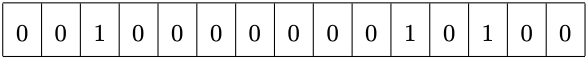
The same procedure is used to insert other elements, each time setting the bits given by the corresponding k indexes.

相同的过程也用于插入其他元素，每次都需要设置对应的 k 个索引的比特位。

In order to query a Bloom filter, say for element x, it suffices to verify if all bits in indexes h1(x), h2(x), . . . , hk(x) are set. If one or more of these bits is not set, then the queried element is definitely not present on the filter. Otherwise, if all these bits are set, then the element is considered to be on the filter. Given this procedure, an error probability exists for positive matches, since the tested indexes might have been set by the insertion of other elements.

为了查询布隆过滤器，比如元素 x，需要验证索引 h1(x)、h2(x)、…, hk(x) 中的所有位是否都被设置（都等于 1 ）。如果这些位中有一个或多个没有被设置，则查询的元素肯定不存在于过滤器中。 否则，如果所有的这些比特位都被设置了，则认为该元素在过滤器中。 基于此过程，匹配命中存在误判率，因为测试（查询）的索引比特位可能会被已插入的其他元素来设置。

With the above setup, all hash functions are used to generate indexes over M. Since these hash functions are independent, nothing prevents collisions in the outputs. In the most extreme case we could have h1(x) = h2(x) = . . . = hk(x). This means that in the general case each element will be described by 1 to k distinct indexes. Although for large values of M a collision seldom occurs, this aspect makes some elements more prone to false positives (and also complicates the analytical derivation of probabilities) [12].

通过上述设置，所有哈希函数都用于在 M 上生成索引。 由于这些哈希函数是相互独立的，因此输出特征值的冲突不可避免。 在最极端的情况下，可能会出现 h1(x) = h2(x) = . . . = hk(x)的情况。 在一般的情况下，每个元素将由 1 到 k 个不同的索引来表示。 尽管当 M 值较大的时候很少会发生碰撞，但这一方面使某些元素更容易出现误报（并且也使概率的分析推导变得更加复杂）[12]。

A variant of Bloom filters [2], which we adopt in this paper, consists of partitioning the M bits among the k hash functions, thus creating k slices of m = M/k bits. In this variant, each hash function hi(), with 1 ≤ i ≤ k, produces an index over m for its respective slice. Therefore, each element is always described by exactly k bits, which results in a more robust filter, with no element specially sensitive to false positives.

我们在本文中采用的布隆过滤器 [2] 是一种变体，包括在 k 个哈希函数中划分 M 位，从而创建 m = M/k 位的 k 个切片。 在这个变体中，每个散列函数 hi() ，1 ≤ i ≤ k，为其各自的切片在 m 上生成一个索引。因此，每个元素总是用精确的 k 位来标示，这将导致过滤器更加健壮，没有对误报特别敏感的元素。

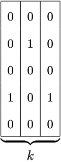
For M = 15 and k = 3 a filter would have 3 slices with 5 bits in each. After insertion of one element, the resulting configuration would have exactly one bit set in each slice. Each slice is depicted here in a column.

对于 M = 15 和 k = 3，过滤器将有 3 个切片，每个切片有 5 位。 插入一个元素后，生成的配置将在每个切片中设置一个位。 每个切片在此处以列的形式描述。

基础变量信息汇总：

• M : 布隆过滤器的大小，单位比特；
• n : 期望写入的元素的数量；
• k : 哈希函数的个数，对应单个元素的索引数量；
• P : 误判率；
• s : 下一个子布隆过滤器容量的增长倍数；
• r : 下一个子布隆过滤器的误判率的变化倍数；

3.1、假阳性

False positives can occur when testing for the presence of a given element x, not present in the filter, and all k bits given by hi(x), 1 ≤ i ≤ k, happen to be set due to the insertion of other elements. Intuitively, if the number of slices k or the slice size m are increased the error probability will decrease.

当测试（查询）给定元素 x 的是否存在时，如果该元素不存在于过滤器中，但是由于 hi(x) 给出的所有 k 个位置（1 ≤ i ≤ k） 恰好被已经插入的其他元素设置了，则可能发生误报。直观地说，如果切片数量 k 或切片大小 m 增加，将会降低误判的概率。

The probability of a given bit being set in a slice is the fill ratio p between the number of set bits in the slice and the slice size m. For a large value m, this ratio will be approximately the same across all slices, and the false positive probability P for the filter will be :

（假设）在切片中设置给定（比特）位的概率是切片中设置位的数量与切片大小 m 之间的填充率 p。 对于较大的值 m，该比率在所有切片中将大致相同，过滤器的误报概率 P 将为：

In the example above, with one element inserted, p is 1/5 and the overall error probability P is (1/5)^3 , thus 0.8%.

在上例中，插入一个元素后，p为1/5，总误判率p为（1/5）^3，因此为0.8%。

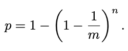
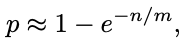
In each slice, the probability that a given 0 bit becomes set after introducing one element is 1/m; it will remain unset with probability 1 − 1/m. If n elements have been inserted, the probability that the given bit is still 0 is (1 − 1/m)^n. Therefore, the probability that a specific bit in a slice is set after n insertions, which is also the expected fill ratio p, is:

在每个切片中，在插入一个元素后给定（比特）位 0 被置的概率是 1/m，未被设置的概率为 1 - 1/m 。 如果已插入 n 个元素，则给定（比特）位仍为 0 的概率为 (1 − 1/m)^n。 因此，在 n 次插入之后，切片中的特定（比特）位被设置的概率，也是预期的填充率 p，为：

3.2、限定错误

From the analysis in the previous section, it is evident that the error probability P increases with n and decreases with m and k. We now determine how to choose k (and thus m) such that, for a given filter size M, we can maximize the number of stored elements n, while keeping the error probability below a certain value P.

从上一节的分析可以看出，错误概率（误判率） P 随着 n 的增加而增加，随着 m 和 k 的增加而减少。 我们现在确定如何选择 k（因此选择 m），使得对于给定的过滤器大小 M，我们可以最大化存储元素的数量 n，同时将错误概率保持在某个 P 值以下。

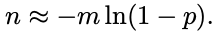
For usable values of m, 1−1/m is almost the same as e^(−1/m) (from the Taylor series expansion); we can use this approximation to obtain:

对于 m 的可用值，1−1/m 与e^(−1/m) 几乎相同（来自泰勒级数展开式）； 我们可以使用这个近似来获得：

from which we obtain:

我们从中获得：

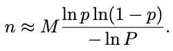
From M = km and P = p^k we obtain m = M * ln(p) / ln(P); therefore:

从 M = km 和 P = p^k 我们得到 m = M * ln(p) / ln(P)； 所以：

For any given error probability P and filter size M, n is maximized by making p = 1/2, regardless of P or M. As p corresponds to the fill ratio of a slice, a filter depicts an optimal use when slices are half full. With p = 1/2 we obtain:

对于任何给定的错误概率（误判率）P 和过滤器大小 M，通过使 p = 1/2 最大化 n，而不管 P 或 M。 由于 p 对应于切片的填充率，因此过滤器描述了切片半满时的最佳使用。 使用p = 1/2，我们得到：

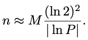
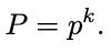
In this expression it is clear that the number of elements n that can be stored, for a given error P, is linear on the filter size M. Finally, from P = p^k and with p = 1/2 we obtain:

在这个表达式中，很明显，对于给定的误差 P，可以存储的元素数量 n 与过滤器大小 M 成线性关系。 最后，从 P = p^k 和 p = 1/2 我们得到：

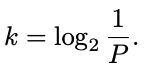
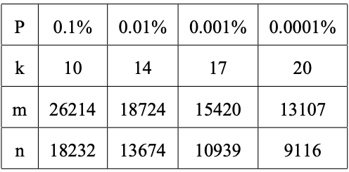
Table 1. Several capacities for a bloom filter with 32 Kilobytes.

表1. 32KB 的布隆过滤器的几种容量

With these formulae it is now possible to determine the optimal filter parameters in order to respect a maximum error probability. For example, to have a maximum error of 0.1% we should have at least 10 slices, since log2 * (1 / 0.001) ≈ 9.96 (2^10 = 1024). If this filter is allocated 32 kilobytes, each slice will have 26214 bits and the filter is predicted to hold up to 18232 elements. See Table 1.

使用这些公式，为了考虑最大错误概率，可以确定最佳过滤器的参数。 例如，要获得 0.1% 的最大误差，我们应该至少有 10 个切片，因为log2 * (1 / 0.001) ≈ 9.96 (2^10 = 1024)。 如果此过滤器分配了 32 千字节，则每个切片将具有 26214 位，并且预计该过滤器最多可容纳 18232 个元素。 参见 表 1。

4、可扩展的布隆过滤器

A Scalable Bloom Filter addresses the problem of having to choose an a priori maximum size for the set, and allows an arbitrary growth of the set being represented. The two key ideas are:

可扩展的布隆过滤器解决了必须事先为集合确定最大容量大小的问题，并允许对应的集合的大小任意增长。 两个关键思想是：

• A SBF is made up of a series of one or more (plain) Bloom Filters; when filters get full due to the limit on the fill ratio, a new one is added; querying is made by testing for the presence in each filter.
• Each successive bloom filter is created with a tighter maximum error probability on a geometric progression, so that the compounded probability over the whole series converges to some wanted value, even accounting for an infinite series.

• SBF 由一系列一个或多个（普通）布隆过滤器组成； 当过滤器由于填充率的限制而被填满时，会添加一个新的； 查询时会验证元素在每个过滤器的存在。
• 每个连续的布隆过滤器都是在几何级数上以更严格的最大错误概率（误判率）创建的，因此整个系列的复合概率收敛到某个想要的值，甚至可以考虑无限系列。

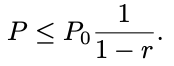
The SBF starts with one filter with k0 slices and error probability P0. When this filter gets full, a new one is added with k1 slices and P1 = P0 * r error probability, where r is the tightening ratio with 0 < r < 1. At a given moment we will have l filters with error probabilities P0, P0 * r, P0 * r^2 , . . . P0 * r^(l−1). The compounded error probability for the SBF will be:

SBF 从一个具有 k0 切片和错误概率（误判率） P0 的过滤器开始。当此过滤器已满时，会添加一个带有 k1 切片和 P1 = P0 * r 错误概率（误判率）的新的过滤器，其中 r 是 0 < r < 1 的紧缩比率（缩小比率）。 在给定时刻，我们将有 l 个错误概率（误判率）为 P0，P0 * r，P0 * r^2 ， . . . P0 * r^(l−1)。 SBF 的复合错误概率为：

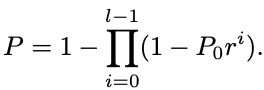
We can use the known approximation:

我们可以使用已知的近似值：

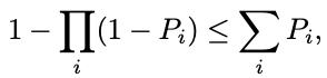
to obtain an upper bound (which will be tight for small Pi):

获得一个上限（对于小的 Pi 来说会很紧）：

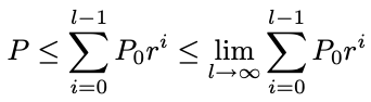
and therefore:

因此：

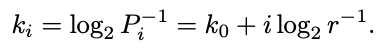
The number of slices for each filter will be:

每个过滤器的切片数将为：

and

并且

To have each ki as an integer, a natural choice will be r = 1/2, resulting in:

要将每个 ki 作为整数，自然选择将是 r = 1/2，结果是：

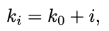
which means an extra slice per new filter. The compounded error probability for the SBF will be bounded by:

这意味着每个新过滤器都有一个额外的切片。 SBF 的复合错误概率将受以下限制：

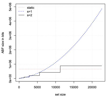
Figure 1. Space usage as a function of set size. Two SBFs, with slice growth factors s = 1 and s = 2, are compared with a static bloom. Both with r = 0.5, m0 = 128 and P = 10^−6 .

图1. 空间使用量与集合大小的函数关系。 将切片生长因子（布隆过滤器的容量增长倍数） s = 1 和 s = 2 的两个 SBF 与静态布隆过滤器进行比较。 都具有 r = 0.5 、 m0 = 128 和 P = 10^−6 。

图1 内容解析：

• 坐标轴信息：
  • 横坐标 （set size） ：数据集大小（数量）；
  • 纵坐标（ABF size in bits）：布隆过滤器的大小，单位比特；
• 含义解释：
  • 静态（普通）布隆过滤器的大小是固定的（根据特定的误判率以及容量确定的），随着数据集的增长，布隆过滤器的大小是没有变化的；
  • 当可扩展布隆过滤器的增长因子为 1 时，下一个创建的布隆过滤器的容量是前一个的 1倍，随着数据集的增长，布隆过滤器的大小呈现 指数增长 的现象；
  • 当可扩展布隆过滤器的增长因子为 2 时，下一个创建的布隆过滤器的容量是前一个的 2倍，随着数据集的增长，布隆过滤器的大小呈现 阶梯状增长 的现象；

Another possibility is to use an r other than 1/2 and round up the resulting ki’s to obtain the number of slices. We will see below that choosing r around 0.8 – 0.9 will result in better average space usage for wide ranges of growth.

另一种可能性是使用 1/2 以外的 r 并四舍五入得到的 ki's 以获得切片数。 我们将在下面看到，在 0.8 - 0.9 之间选择 r 将导致更大范围的增长更好的平均空间使用率。

4.1、可扩展的增长

The estimation of the set size that is to be stored in a filter may be wrong, possibly by several orders of magnitude. We may also want to use not much more memory than needed at a given time, and start a filter with a small size. Therefore, a SBF should be able to adapt to variations in size of several orders of magnitude in an efficient way.

预估的存储在过滤器中的集合大小可能是错误的，有可能相差几个数量级。 可能我们还希望在给定时间内使用不超过所需的内存，并启动一个小尺寸的过滤器。 因此，SBF 应该能够以有效的方式适应几个数量级的大小变化。

When a new filter is added to a SBF, its size can be chosen orthogonally to the required false positive probability. A flexible growth can be obtained by making the filter sizes grow exponentially. We can have a SBF made up of a series of filters with slices having sizes m0, m0 * s, m0 * s^2 , . . . , m0 * s^(l−1) .

当一个新的过滤器被添加到一个 SBF 时，它的大小可以与所需的误报概率正交地选择（正相交？）。 通过使过滤器的大小呈指数增长，可以获得灵活的增长。 我们可以有一个由一系列过滤器组成的 SBF，这些过滤器的切片大小为 m0、m0 * s、m0 * s^2、.. . . , m0 * s^(l−1) 。

Given that filters stop being used when the fill ratio reaches 1/2, filter i will hold approximately:

鉴于过滤器在填充率达到 1/2 时停止使用，过滤器 i 将保持大约：

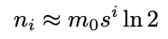
elements. The SBF with l stages will hold about:

元素。 具有 l 个阶段的 SBF 将保持大约：

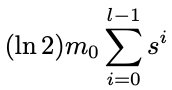
elements. This geometric progression allows a fast adaptation to set sizes of different orders of magnitude. A practical choice will be s = 2, which preserves mi as a power of 2, if m0 already starts as such; this is useful, as the range of a hash function is typically a power of 2.

元素。 这种几何级数允许快速适应不同数量级的设置大小。 一个实际的选择是 s = 2，如果 m0 已经开始这样，它会将 mi 保留为 2 的幂； 这很有用，因为散列函数的范围通常是 2 的幂。

In general, other values of s may be used. Figure 1 shows the required size for the SBF as a function of set size, n, for s = 1 and s = 2. The case s = 1 gives a constant m in all stages; this case is not feasible as it would lead to much inefficiency, as the number of stages required grows linearly with set size, and in each stage an extra slice would be required (for r = 1/2); this would result in rapidly increasing space per element and computational cost for the hash functions. For s = 2 we can see that not only the number of stages remains low, as it increases logarithmically with the set size, but also the space required for the 22624 element set is only slightly more than for a static filter dimensioned for that size.

通常，可以使用其他值的s。 图 1 显示了 SBF 所需的大小作为集合大小 n 的函数，对于 s = 1 和 s = 2。 当 s = 1 在所有阶段给出一个常数 m； 这种情况是不可行的，因为它会导致效率低下，因为所需的阶段数会随着集合大小线性增长，并且在每个阶段都需要一个额外的切片（对于 r = 1/2）； 这将导致每个元素的空间和散列函数的计算成本迅速增加。 对于s = 2，我们可以看到不仅阶段数仍然很低，因为它随着集合大小呈对数增加，而且22624元素集所需的空间仅比静态过滤器尺寸略多 对于那个尺寸。

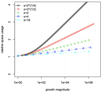
Figure 2. Relative space usage with respect to a static filter as a function of set growth. With r = 0.5 and P = 10^−6 .

图 2. 相对于静态布隆过滤器的相对空间使用率作为集合增长的函数。 使用 r = 0.5 和 P = 10^−6 。

图2 内容解析：

• 坐标轴信息：
  • 横坐标 （growth magnitude） ：增长幅度；
  • 纵坐标（relative space usage）：相对空间使用量，相比静态（普通）布隆过滤器；
• 含义解释：
  • 观察可扩展的布隆过滤器的下一个子布隆过滤器的误判率是上一个的 0.5 倍，并且误判率为 10^-6 = 0.000001 的情况下；

To better understand adaptation to growth, we should not plot space usage against an absolute set size, but against the relative growth over the initial size. We should have a scale-free graph telling us how much space will be used according to the orders of magnitude in size the filter has to adapt to. Figure 2 plots the space usage relative to a static filter dimensioned for the required size. Here we can see that if the set had to grow by 6 orders of magnitude, for s = 2 the SBF would use about twice the space of a static filter exactly dimensioned for the final size, and fors = 4 about 50% more space. In terms of space usage we can see that practical values of s like 2, 4 or above can be chosen, and values below 2 and approaching 1 will give progressively worse results.

为了更好地理解对增长的适应，我们不应该根据绝对集合大小绘制空间使用情况，而是针对初始大小的相对增长。 我们应该有一个无标度图，告诉我们根据过滤器必须适应的大小数量级将使用多少空间。 图 2 绘制了相对于所需尺寸的静态过滤器的空间使用情况。 在这里我们可以看到，如果集合必须增长 6 数量级，对于 s = 2，SBF 将使用大约两倍的静态过滤器空间，该静态过滤器的尺寸恰好适合最终尺寸，而对于s = 4 约 50% 更多空间。 在空间使用方面，我们可以看到 s 的实际值可以选择，例如 2、4 或更高，低于 2 和接近 1 的值会产生越来越差的结果。

Another aspect to consider in the choice of s is the number of stages required for the SBF. Figure 3 plots the number of stages as a function of s, for two cases of set growth: 10^2 and 10^6. This figure confirms that s should not be chosen near 1 and that the practical choice of s as a power of two is a sensible one with this respect.

在选择 s 时要考虑的另一个方面是 SBF 所需的级数。 图 3 将阶段数绘制为 s 的函数，对于两种集合增长情况：10^2 和 10^6。 这个数字证实了 s 不应该选择在 1 附近，并且在这方面实际选择 s 作为 2 的幂是一个明智的选择。

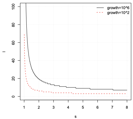
Figure 3. Number of stages as a function of s.

图 3. 阶段数作为 s 的函数。

图3 内容解析：

• 坐标轴信息：
  • 横坐标 （s） ：下一个子布隆过滤器容量的增长倍数；
  • 纵坐标（l）：子布隆过滤器的数量；

From these figures one could be led to think that the larger the s the better. However, as s tends to infinity, each successive stage of the SBF will take considerably more space which will remain poorly used for considerably more time until it gets full. A better criterion is to consider the average space usage over the lifetime of the SBF from an empty set until the final set size. Figure 4 plots this average space usage relative to a static filter (dimensioned for the final set size), as a function of s, for several combinations of error probability (10^−3 and 10^−6) and set growth (10^2 and 10^6 ). These curves cover a wide range of scenarios; they show that, as long as s is not very close to 1, increasing s is not profitable.

从这些数字可以导致人们认为 s 越大越好。 然而，由于 s 趋于无穷大，SBF 的每个连续阶段将占用相当多的空间，这些空间将在相当长的时间内保持不良使用状态，直到它被填满。 更好的标准是考虑 SBF 生命周期内从空集到最终集大小的平均空间使用情况。 图 4 绘制了相对于静态过滤器的平均空间使用情况（根据最终集大小确定），作为 s 的函数，对于错误概率的几种组合（10^−3 和 10^−6 ) 并设置增长（10^2 和 10^6）。 这些曲线涵盖了广泛的场景； 他们表明，只要 s 不是很接近 1，增加 s 是无利可图的。

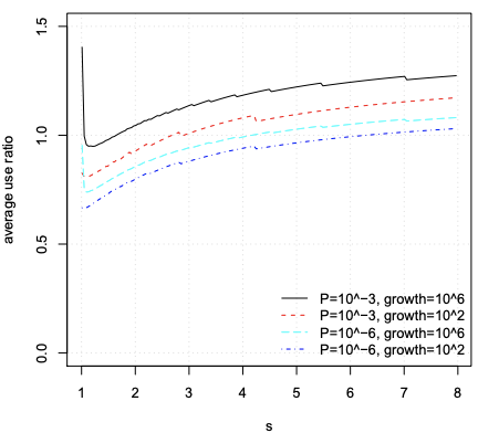
Figure 4. Average relative space usage as a function of s, for different combinations of set growth and P, for optimal r.

图 4. 对于集合增长和“P”的不同组合，作为 s 函数的平均相对空间使用率，以获得最佳 r。

图4 内容解析：

• 坐标轴信息：
  • 横坐标 （s） ：下一个子布隆过滤器容量的增长倍数；
  • 纵坐标（average use ratio）：平均使用率；

Combining these two criteria, i.e. average space and number of stages, with the convenience of having a power of two, we can conclude that 2 or 4 will be a sensible choice for s. To keep the number of stages small, we can choose s = 2 if we expect a small set growth and s = 4 if we expect a larger growth.

结合这两个标准，即平均空间和阶段数，加上 2 的幂的便利性，我们可以得出结论，2 或 4 将是 s 的明智选择。 为了保持阶段的数量较少，如果我们期望小的集合增长，我们可以选择s = 2，如果我们期望更大的增长，我们可以选择s = 4。

4.2、选择错误判断比例

The other parameter of a SBF that we need to choose is the error probability ratio r. We can choose values other than 0.5 and round up the resulting number of slices for stage i:

我们需要选择的 SBF 的另一个参数是错误概率比 r。 我们可以选择 0.5 以外的值，并对阶段 i 的切片数进行四舍五入：

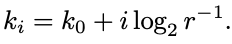
Figure 5 compares the space usage as a function of set growth for different combinations of P and r. It shows that if we use an r larger than 0.5, although we start by using more space (we need more initial slices, k0, as P0 needs to be smaller for the geometric series to converge to the same P), after some point we end up using less and less space as the set grows, as we add slices less frequently at each new stage. It specially pays to use a large r for a tighter error probability P, as the few extra slices needed initially will be a small overhead over the already large number of slices needed for r = 0.5.

图 5 比较了 P 和 r 的不同组合的空间使用作为集合增长的函数。 它表明，如果我们使用大于 0.5 的 r ，尽管我们从使用更多空间开始（我们需要更多初始切片， k0，因为 P0 需要更小才能使几何级数收敛到 相同的P），在某个点之后，随着集合的增长，我们最终使用的空间越来越少，因为我们在每个新阶段添加切片的频率越来越低。 使用较大的 r 来获得更严格的错误概率 P 是特别值得的，因为最初需要的几个额外切片将比r = 0.5 所需的已经大量切片的开销小。

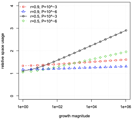
Figure 5. Relative space usage as a function of growth, for different combinations of P and r and s = 2.

图 5. 对于 P 和 r 以及 s = 2 的不同组合，作为增长函数的相对空间使用情况。

图5 内容解析：

• 坐标轴信息：
  • 横坐标 （growth magnitude） ：增长幅度；
  • 纵坐标（relative space usage）：相对空间使用量，相比静态（普通）布隆过滤器；

Figure 4 shows average relative space usage, calculated for the optimal r that minimizes average space, for each combination of growth and s values (the optimal r does not depend on P).

图 4 显示了平均相对空间使用情况，为最小化平均空间的最佳 r 计算，对于增长和s值的每个组合（最佳r不依赖于P）。

In order to select an appropriate value for r we can observe how the optimal r behaves for different growth and s values. Figure 6 shows the optimal r as a function of set growth, for three different values of s (√2, 2, 4). Considering the choice of s = 2 for small expected growth and s = 4 for larger growth, one can see that r around 0.8 – 0.9 is a sensible choice, that gives better space usage than the natural r = 1/2.

为了为 r 选择一个合适的值，我们可以观察最佳 r 对于不同的增长和 s 值的表现。 图 6 显示了最优 r 作为集合增长的函数，对于 s (√2, 2, 4) 的三个不同值。 考虑到较小的预期增长选择 s = 2 和较大增长的 s = 4 ，可以看出 r 大约在 0.8 – 0.9 是一个明智的选择，它比自然的 r = 1/2。

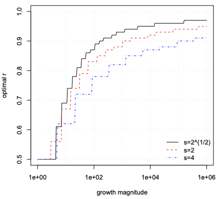
Figure 6. Optimal r as a function of growth magnitude, for s ∈ {√ 2, 2, 4} and P = 10^−6 .

图 6. 对于 s ∈ {√ 2, 2, 4} 和 P = 10^−6，最佳 r 作为增长幅度的函数。

图6 内容解析：

• 坐标轴信息：
  • 横坐标 （growth magnitude） ：增长幅度；
  • 纵坐标（optimal r）：最优的 r ；

5、结论

Bloom Filters and the existing variants require a priori dimensioning of the maximum size of the set to be stored in the filter. Given that it is not always possible to know in advance how many elements will need to be stored, this leads to over-dimensioning the filters, possibly by several orders of magnitude.

布隆过滤器和现有变体需要事先确定要存储在过滤器中的集合的最大大小。 考虑到（用户）并不总能提前知道需要存储多少元素，这就会导致布隆过滤器尺寸过大，可能还会增加几个数量级。

In this paper we have introduced Scalable Bloom Filters (SBF), a mechanism that allows representing sets without having to know a priori the maximum set size and yet being able to choose from the start the maximum false positive probability. The mechanism adapts to set growth by using a series of classic Bloom Filters of increasing sizes and tighter error probabilities, added as needed.

在本文中，我们介绍了可扩展的布隆过滤器（SBF），一种允许表示集合的机制，而无需事先知道最大集合大小，并且能够从一开始就选择最大误报概率。 该机制通过使用一系列经典的布隆过滤器来适应集合增长，这些布隆过滤器的大小越来越大，错误概率越来越小，根据需要添加。

A SBF is parameterized not only by the initial size and error probability but also by the growth rate of the size and by the error probability tightening rate. In this paper we have studied the impact of these parameters on space usage and shown how they can be chosen for a range of scenarios.

SBF 不仅由初始大小和错误概率参数化，而且由大小的增长率和错误概率收紧率参数化。 在本文中，我们研究了这些参数对空间使用的影响，并展示了如何为一系列场景选择它们。

参考文献

[1]. B. H. Bloom, Space/time trade-offs in hash coding with allowable errors, Commun. ACM 13 (7) (1970) 422–426.
[2]. F. Chang, W. chang Feng, K. Li, Approximate caches for packet classification, in: Proc. of the 23rd Annual Joint Conference of the IEEE Computer and Communications Societies (INFOCOM 2004), IEEE, 2004.
[3]. P. Reynolds, A. Vahdat, Efficient peer-to-peer keyword searching., in: M. Endler, D. C. Schmidt (Eds.), Middleware, Vol. 2672 of Lecture Notes in Computer Science, Springer, 2003, pp. 21–40.
[4]. S. C. Rhea, J. Kubiatowicz, Probabilistic location and routing., in: Proc. of the 21st Annual Joint Conference of the IEEE Computer and Communications Societies (INFOCOM 2002), 2002.
[5]. L. Fan, P. Cao, J. Almeida, A. Z. Broder, Summary cache: a scalable wide-area web cache sharing protocol, IEEE/ACM Trans. Netw. 8 (3) (2000) 281–293.
[6]. L. F. Mackert, G. M. Lohman, R* optimizer validation and performance evaluation for distributed queries, in: Proceedings of the Twelfth International Conference on Very Large Data Bases (VLDB ’86), Morgan Kaufmann Publishers Inc., San Francisco, CA, USA, 1986, pp. 149–159.
[7]. A. Broder, M. Mitzenmacher, Network applications of bloom filters: A survey, in: Proc. of Allerton Conference, 2002.
[8]. S. Cohen, Y. Matias, Spectral bloom filters, in: Proceedings of the 2003 ACM SIGMOD international conference on Management of data (SIGMOD ’03), ACM Press, New York, NY, USA, 2003, pp. 241–252.
[9]. U. Manber, S. Wu, An algorithm for approximate membership checking with application to password security, Inf. Process. Lett. 50 (4) (1994) 191–197.
[10]. S. Dharmapurikar, P. Krishnamurthy, D. E. Taylor, Longest prefix matching using bloom filters, in: Proceedings of the 2003 conference on Applications, technologies, architectures, and protocols for computer communications (SIGCOMM ’03), ACM Press, New York, NY, USA, 2003, pp. 201–212.
[11]. M. Mitzenmacher, Compressed bloom filters, IEEE/ACM Trans. Netw. 10 (5) (2002) 604–612.
[12]. P. Bose, H. Guo, E. Kranakis, A. Maheshwari, P. Morin, J. Morrison, M. Smid, Y. Tang, On the false-positive rate of bloom filters, submitted to Information Processing Letters, available at http://citeseer.ist.psu.edu/649161.html (2004).